Typical Serviced Image
A typical serviced satellite image (bought or downloaded) includes several processing steps. From the raw image (Level 0), data are calibrated into units of physical reflectance (called Level 1 processing), and the image is geolocated and ortho-rectified following an elevation model of the terrain, Ground Control Points (GCP), or a geodetic reference frame (e.g., Mercator). Over large areas, several captures may need to be stitched together. This product is usually referred to as Level 2 or similar. In many cases, the end user will only see the final image, either in a report or as an interactive map on the web, such as the maps in this report.
Data Processing Levels
The following paragraph and table explore the different levels of data processing that are done specifically by NASA, but also apply to the industry at large.
NASA’s Earth Observing System Data and Information System (EOSDIS) data products are processed at various levels ranging from Level 0 to Level 4. Level 0 products are raw data at full instrument resolution. At higher levels, the data are converted into more useful parameters and formats. All EOS instruments must have Level 1 Standard Data Products (SDPs); most have SDPs at Level 2 and Level 3; and many have Level 4 SDPs. Some EOS Interdisciplinary Science Investigations also have generated Level 4 SDPs. Specifications for the set of SDPs to be generated are reviewed by the Earth Observing System Project Science Office (EOSPSO) and NASA Headquarters to ensure completeness and consistency in providing a comprehensive science data output for EOS. Standard data products are produced at NASA’s Distributed Active Archive Centers (DAACs) or Science Investigator-led Processing Systems (SIPS).
| Data Level | Description |
|---|---|
| Level 0 | Reconstructed, unprocessed instrument and payload data at full resolution, with any and all communications artifacts (e.g., synchronization frames, communications headers, duplicate data) removed. (In most cases, NASA’s EOS Data and Operations System [EDOS] provides these data to the DAACs as production data sets for processing by the Science Data Processing Segment [SDPS] or by one of the SIPS to produce higher-level products.) |
| Level 1A | Level 1A (L1A) data are reconstructed, unprocessed instrument data at full resolution, time-referenced, and annotated with ancillary information, including radiometric and geometric calibration coefficients and georeferencing parameters (e.g., platform ephemeris) computed and appended but not applied to L0 data. |
| Level 1B | L1B data are L1A data that have been processed to sensor units (not all instruments have L1B source data). |
| Level 1C | L1C data are L1B data that include new variables to describe the spectra. These variables allow the user to identify which L1C channels have been copied directly from the L1B and which have been synthesized from L1B and why. |
| Level 2 | Derived geophysical variables at the same resolution and location as L1 source data. |
| Level 2A | L2A data contains information derived from the geolocated sensor data, such as ground elevation, highest and lowest surface return elevations, energy quantile heights (“relative height” metrics), and other waveform-derived metrics describing the intercepted surface. |
| Level 2B | L2B data are L2A data that have been processed to sensor units (not all instruments will have a L2B equivalent). |
| Level 3 | Variables mapped on uniform space-time grid scales, usually with some completeness and consistency. |
| Level 3A | L3A data are generally periodic summaries (weekly, ten-day, monthly) of L2 products. |
| Level 4 | Model output or results from analyses of lower-level data (e.g., variables derived from multiple measurements). |
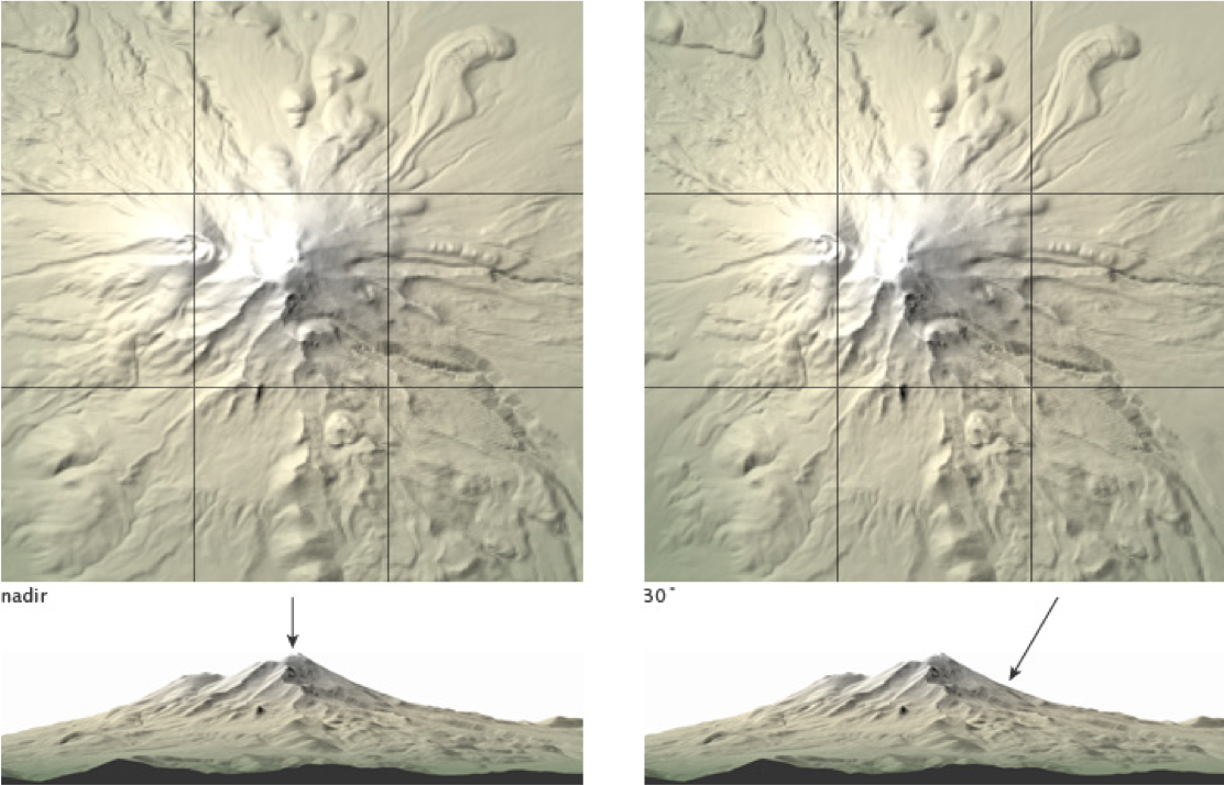
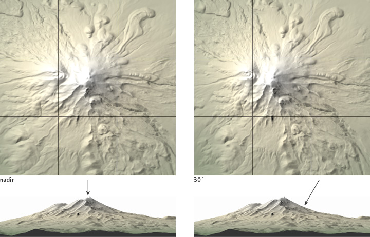
Orthorectification
Imagery has an amazing amount of information, but raw aerial or satellite imagery cannot be used in a GIS until it has been processed such that all pixels are in an accurate (x,y) position on the ground. Photogrammetry is a discipline, developed over many decades, for processing imagery to generate accurately georeferenced images, referred to as orthorectified images (or sometimes simply orthoimages). Orthorectified images have been processed to apply corrections for optical distortions from the sensor system, and apparent changes in the position of ground objects caused by the perspective of the sensor view angle and ground terrain.
Atmospheric Compensation
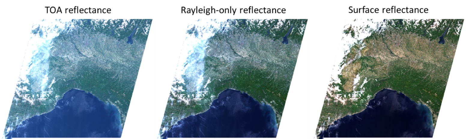
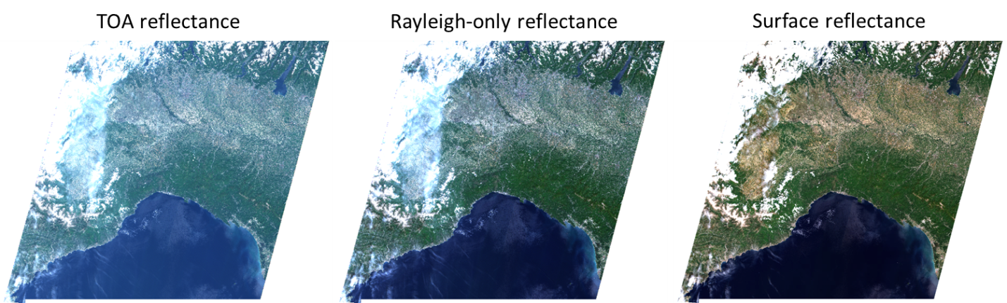
There are three main types of Atmospheric Compensation algorithms used by imagery providers. They all aim to remove atmospheric effects from raw imagery but go about solving the problem through different methods.
Top-of-atmosphere (TOA) reflectance performs a normalization for solar energy. TOA normalizes the pixels values to the 0.0-1.0 range to reduce variability between images. Because the information needed to convert digital numbers (DN) to TOA reflectance values is known, this transformation is very fast and fully automated. The main limitations of TOA reflectance are the remaining effects of Rayleigh scattering (which results in bluish images), aerosol absorption and scattering phenomena (which result in non-uniform, decreased image visibility).
Rayleigh-only reflectance accounts for the systematic properties of the atmosphere by removing the Rayleigh scattering component (a result of the interaction of sunlight with molecules in the atmosphere) from imagery. Again, the transformation is very fast and fully automated. In cases of very low aerosol loads, Rayleigh-only reflectance produces images that are less blue than TOA reflectance, but the effects of haze variability remain visible.
Surface reflectance compensates for atmospheric absorption and scattering phenomena on a pixel-by-pixel basis. It approximates what would be measured by a sensor held just above the Earth surface, without any alterations from the atmosphere. Of these three choices, surface reflectance oftentimes provides the best visual experience.