Spectral Bands
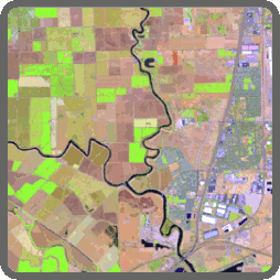
A simple form of image interpretation involves assigning invisible light bands to red, green, and blue channels to create a false color image, commonly referred to as ‘band combinations’. Band combinations are used to highlight the presence of certain materials and/or minimize the representation of other features. The most common band combination is Natural Color and is used to mimic what the human eye would see over a given region, another common combination is Color Infrared which highlights the presence of vegetation.
False Color
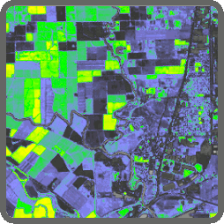
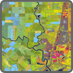
False color images can distinguish muddy water from muddy land, pinpoint fires, or clearly show the extent of a growing city. The example combines the moisture sensitivity of mid-Infrared reflectance with the vegetation sensitivity of near-infrared to highlight agricultural fields.
In this imagery over rural Uganda, near-infrared sensors augment imagery to highlight vegetation (False Color) and to measure the health of that vegetation (NDVI). These images show a range of imagery resolutions from different growing seasons.
Each sensor has a specific set of spectral bands designed for the mission of the satellite. While some sensors may have only 3 or 4 bands, others may have dozens, or hundreds (these are called hyperspectral sensors). Many earth-observing satellites include bands that fall within commonly used ‘windows’, such as “red” or “near-infrared”.
| Common Name | Band Range (μm) | Landsat 5 | Landsat 7 | Landsat 8 | Sentinel 2 | MODIS |
|---|---|---|---|---|---|---|
| Coastal | 0.40 - 0.45 | 1 | 1 | |||
| Blue | 0.45 - 0.5 | 1 | 1 | 2 | 2 | 3 |
| Green | 0.5 - 0.6 | 2 | 2 | 3 | 3 | 4 |
| Red | 0.6 - 0.7 | 3 | 3 | 4 | 4 | 1 |
| Pan | 0.5 - 0.7 | 8 | 8 | |||
| NIR | 0.77 - 1.00 | 4 | 4 | 5 | 8 | 2 |
| Cirrus | 1.35 - 1.40 | 9 | 10 | 26 | ||
| SWIR16 | 1.55 - 1.75 | 5 | 5 | 6 | 11 | 6 |
| SWIR22 | 2.1 - 2.3 | 7 | 7 | 7 | 12 | 7 |
| LWIR | 10.5 - 12.5 | 6 | 6 | 10, 11 | 31, 32 |
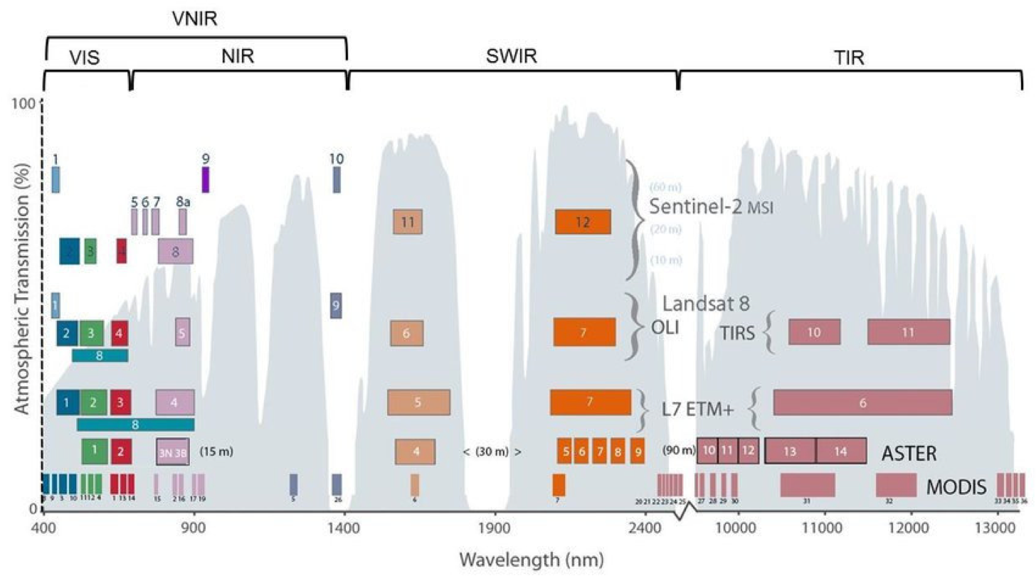
While the individual band specifications can vary, a “blue” band on any sensor is going to roughly fall within 0.45 and 0.5 microns.
- Coastal: A coastal band is used for imaging shallow water, detecting fine particles in the atmosphere (aerosols), and measuring subtle changes in ocean color.
- Red, Green, Blue: Covering the human visible range of 0.4 - 0.7 microns, these bands are the ones most often used for visualization.
- Pan: A panchromatic is a single band that covers the entire visible range, thereby creating a “black & white” image. Pan bands are useful due to their increased sensitivity (from the larger spectral range), and are also frequently higher resolution than other spectral bands on the same sensor. High resolution pan bands can be used to pan-sharpen on other spectral bands to increase their apparent resolution.
- NIR: The Near-infrared is beyond the range of human vision but is widely used in a variety of applications it’s ability to separate out water and vegetation.
- Cirrus: A spectral band in this range has become common on more recent sensors due to it’s ability to detect high altitude clouds (i.e., cirrus clouds) that are invisible in other bands.
- Short Wave Infrared (SWIR): Imaging systems using the short-wave infrared (SWIR) wavelength bands offer unique remote sensing capabilities, such as material detection and smoke penetration overcoming challenges in measurement, inspection, and process-monitoring applications often impossible with other technologies.
- Long Wave Infrared (LWIR): The long-wave infrared region is used to measure temperature on land or water. Some LWIR sensors cover the entire region from 10.5 to 12.5 microns, while others such as Landsat-8, will split the region up into 2 bands.
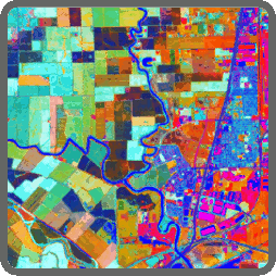
These different spectral bands can be combined in different ways to enhance the contrast between different categories of interest. The most common is to use the red, green, and blue bands to create a natural color image, like what would be seen with the naked eye. See the following chart for common band combinations that bring about specific insights in the data.
Types of Spectal Bands Windows:
| Combination Name | Band 1 | Band 2 | Band 3 |
|---|---|---|---|
| Natural Color | red | green | blue |
| Urban False Color | swir22 | swir16 | red |
| Agriculture | nir | red | green |
| Atmospheric Penetration | swir22 | swir16 | nir |
| Healthy Vegetation | nir | swir16 | blue |
| Land/Water | nir | swir16 | red |
| Natural With Atmospheric Removal | swir22 | nir | green |
| Vegetation Analysis | swir16 | nir | red |
Mathematic spectral transformations
In addition to false color composition, spectral bands can be combined mathematically to emphasize a particular set of characteristics. These techniques may draw from all relevant bands, rather than the three band ‘limit’ set by human vision, to draw out very specific characteristics. This generally demands greater processing of the raw data to minimize noise across the deeper image stack. Mathematical transformations can be combined with ground data and well-developed algorithms to answer more quantitative questions. While false color can be used to detect the subjective health of agriculture, the proper mathematic transformations might be able to measure the health of each field using a transferrable metric. While false color composites can distinguish mud from water, a mathematic transformation could measure how wet the mud is.
Common use cases of vegetation indices are vegetation mapping and monitoring, biodiversity assessments, forest degradation assessments, biomass mapping, crop condition monitoring and predicting crop yield, and carbon capture assessment. Other common indices have been developed to measure burn severity, geologic qualities such as the presence of certain minerals, water turbidity, mud, snow, and more.
Vegetation and other Indices
Synthesizing data from multiple spectral bands, through ratio or coefficient-based transformations, can produce indices that can be used to compare every point in an image on the same scale. The most common indices, such as Normalized Difference Vegetation Index (NDVI) and Enhanced Vegetation Index (EVI), measure vegetation health and can be used to distinguish between types of plants. Soil Adjusted Vegetation Index (SAVI) and its counterparts OSAVI and GSAVI suppresses the effects of soil which can lead to erroneous NDVI calculations in areas with sparse vegetation. A comprehensive list of vegetation indices and their formulas can be found at l3harrisgeospatial.co. Common use cases of vegetation indices are vegetation mapping and monitoring, biodiversity assessments, forest degradation assessments, biomass mapping, crop condition monitoring and predicting crop yield, and carbon capture assessment. Other common indices have been developed to measure burn severity, geologic qualities such as the presence of certain minerals, water turbidity, mud, snow, and more. Normalized Difference Water Index (NDWI) and Normalized Difference Snow Index (NDSI) – Commonly used for water mapping and water quality monitoring, change detection, flood monitoring and damage assessment, snow and ice mapping and monitoring. Normalized Difference Built-up Index (NDBI) – emphasizes manufactured and built-up environments in imagery.
Principle Component Analysis
Another image synthesis technique, Principle Component Analysis (PCA), decorrelates the data within each spectral band, such that the most common characteristics of all bands are placed in the highest category and less common characteristics are placed in lower categories, until all variance is explained. It is invaluable for exploration of data and landscape characteristics, simultaneously drawing attention to the most noteworthy and best-hidden features in a scene.
Kauth-Thomas
KT-Transformations are a type of PCA, which, rather than being data-driven, combine information from multiple bands using specially developed coefficients to create the biophysically meaningful variables of Brightness, Greenness, and Wetness- essential components of a landscape.